STS Quick Start
This tutorial briefly walks through the general work flow and features of STS. For a more comprehensive description of STS, see the STS Manual.
Overview
In this tutorial, you will learn how to get STS up and running, load DNA sequences into the program, perform a basic pattern search of the DNA sequences, and perform a traversal of the data set.
What is STS?
STS is a tool for searching and analyzing very large DNA sequence data sets. STS indexes the input DNA sequences into data structures called suffix trees, which allow STS to perform extremely fast pattern searches.
What can I do with STS?
With STS, you can can perform extremely fast searches of a DNA sequence data set for specific motifs, with optional wildcards and mismatches.
You can also traverse the data set to glean information such as the longest subsequences common to a certain number of input sequences.
How do I get started?
In order to run STS, you will need to have installed Java Web Start, which is done automatically when you install Java.
If Java is not already installed on your computer, you can get it here.
Once you have Java Web Start, the next step is to download STS. If you are not immediately prompted to open the sts.jnlp file after the download finishes, you can launch it manually, either by double-clicking it or typing javaws path/to/sts.jnlp into a terminal session (/Applications/Utilities/Terminal.app on OS X).
You will be greeted by a window that looks like this:

In order to start analyzing sequences, we need to import the sequences, and build the corresponding suffix tree indexes.
Importing the sequences
Click on the Import fasta button in the top left corner, select one or more FASTA-formatted sequence files (multiple files can be selected using cmd-click on OS X or ctrl-click on GNU/Linux), and hit enter.
You will be prompted to enter a name for the suffix tree. This name will be used to create the folder on disk that holds the suffix tree files.
Once you have entered a name for the suffix tree, a status bar will appear and a short load time will follow, which is usually only a few seconds.
The screen should now look something like this:
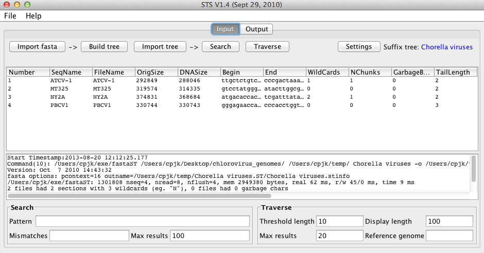
Each input sequence is given its own row, and information about each sequence is displayed in the corresponding columns, the meanings of which can be found here.
Each input sequence is associated with a unique number, which is used to identify the sequence when analyses are run.
Building the suffix trees
Once you are satisfied with the sequences that you have uploaded, hit the build tree button.
A status bar will appear, and the STS will begin to construct the suffix tree index of the input sequences.
Depending on the size and number of input sequences, the build time can range from less than one second to several minutes. The sequences shown, with a total size of approximately 1.3 million nt, took about 3 seconds to index.
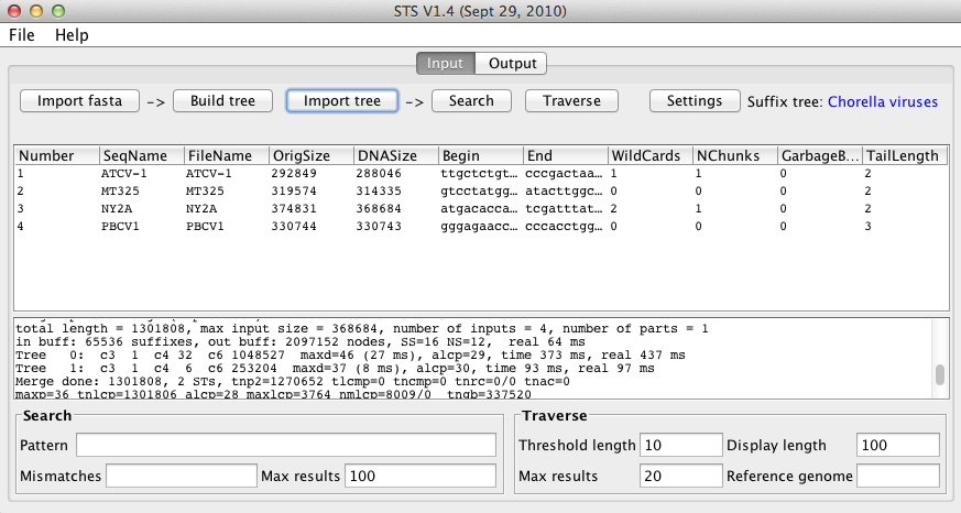
Once the process has finished, the window will look like this:
Performing a pattern search
Now that the sequences have been indexed, we can begin to analyze the sequences.
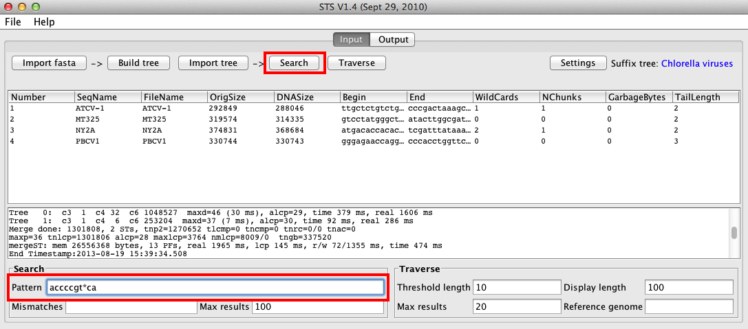
One of STS’s strengths is that searches can be conducted very quickly. Let’s perform a basic search for a the motif “accccgt*ca”, where “*” represents a wildcard (any of a, c, g, or t).
To do this, we will enter the search pattern into the Pattern box in the Search section at the bottom of the window, and click the Search button at the top of the window:
When the search finishes, STS will display the results in a table in the Output window, shown below:
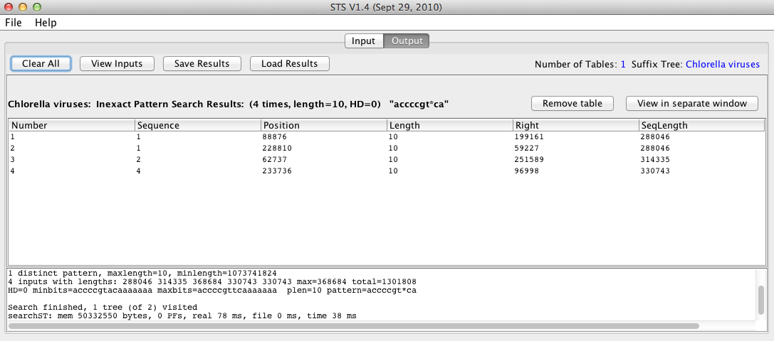
Each row in the results table corresponds to a single match, and information about each match is displayed in different columns, the meanings of which can be found here.
In this case, the motif was found a total of 4 times in the input data set – twice in sequence 1, and once in each of sequences 2 and 4. The names corresponding to the sequence column numbers can be viewed by clicking View Inputs at the top of the screen.
Traversing the data set
Next, let’s perform a traversal of the data set, which will provide an overview of some of the most common motifs present across the data set.
Navigate back to the Input pane by clicking the Input button at the top of the window, and click the Traverse button at the top of the window.
The Output pane will appear again, but there are now two new results tables, in addition to the table from the previous pattern search:
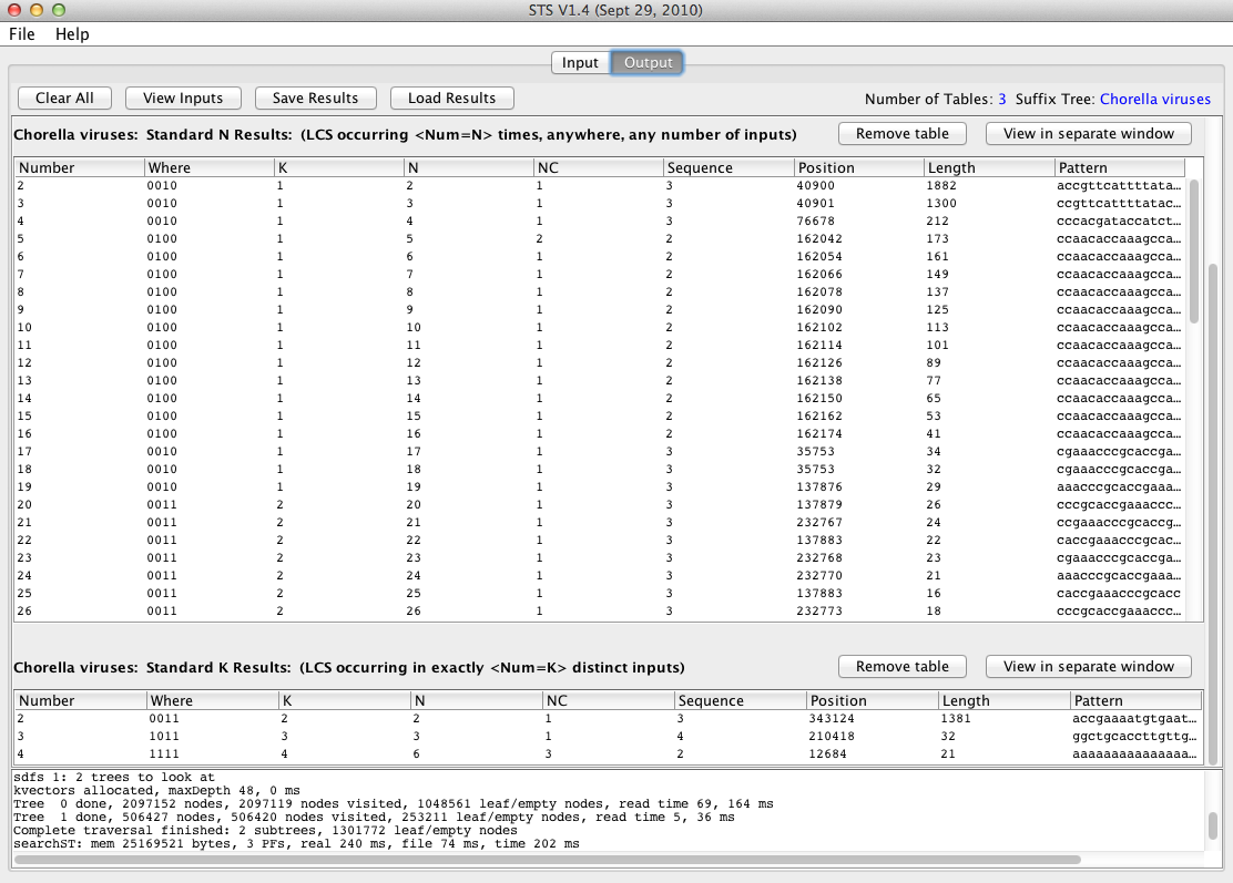
The Standard N Results table shows the longest patterns occurring N times in the data set, for different values of N.
The Standard K Results table shows the longest patterns occurring in K different sequences.
Each row corresponds to a single match.
The meanings of the different columns can be found here
Each time an additional search or traversal is performed, a new results table is added to the output window. You can remove unwanted tables by clicking the remove table button above the corresponding table.
Although we conducted both the search and traversal over the entire data set, you can restrict the sequences that are searched or traversed through the Traverse settings or by specifying special patterns in the Search box, respectively, both of which are located on the Input pane.